During my school days, one day evening my mathematics professor was teaching me about Fourier transform.

My friend asked me: Where do we use this Fourier transform?

I also had the same doubt at that time. But when I stepped into a machine learning field, I got to know the actual use of the Fourier transform.

What is Fourier Transform?

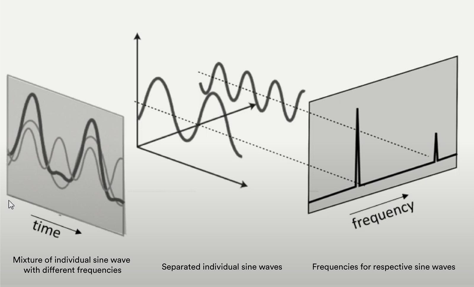
Fourier transform breaks a function (signal) into an alternate representation. In other words, Fourier transforms show any signal can be reconstructed by summing up individual sines and cosines together.

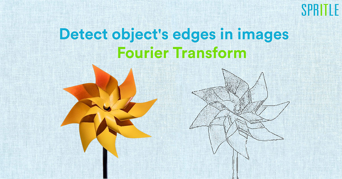
How is Fourier transform relevant for image processing?

The main use of the Fourier transform is separating the signal, when we apply Fourier transform into the image, the high frequency, and low-frequency points will be separated.

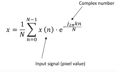
Fourier transforms have two types: continuous and discrete functions, here we are working with digital images so, digital images have discrete signals or discrete signals, so we have to use discrete Fourier transform.

FFT — Fast Fourier Transform

“Fast Fourier Transform” (FFT) is an important measurement method in the science of audio and acoustics measurement. It converts a signal into individual spectral components and thereby provides frequency information about the signal. FFTs are used for fault analysis, quality control, and condition monitoring of machines or systems. This article explains how an FFT works, the relevant parameters, and their effects on the measurement result.

Strictly speaking, the FFT is a fast computation algorithm for discrete Fourier transform (DFT). A signal is sampled over a period of time and divided into its frequency components. These components are single sinusoidal oscillations at distinct frequencies each with its own amplitude and phase. This transformation is illustrated in the following diagram. Over the time period measured, the signal contains 3 distinct dominant frequencies.

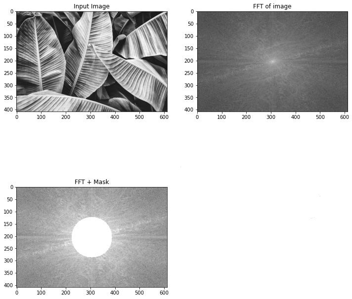
When we apply FFT (Fast Fourier Transform) to the input image center regions are represented by low-frequency components and outer regions are represented by high-frequency components.

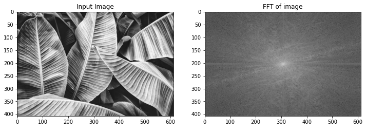
Edges are high-frequency components in the images so we apply the mask(low pass filter)in the center region of low-frequency components to get better edge detection.

Let’s Code

Import the necessary python packages

import cv2
from matplotlib import pyplot as plt
import numpy as np 

load an image

img = cv2.imread( " image path", 0)

Image output is a 2D complex array. 1st channel is real and 2nd imaginary. For FFT (fast Fourier transform) in OpenCV, the input image needs to be converted to float32 and the output will be complex output, which means we need to extract the magnitude out of this Complex number.

dft = cv2.dft(np.float32(img), flags=cv2.DFT_COMPLEX_OUTPUT)

Rearranges a Fourier transform by shifting the zero-frequency component to the center of the array. Otherwise, it starts at the top left corner of the image (array)

dft_shift = np.fft.fftshift(dft)

The magnitude of the function is 20. log(abs(f)), For values that are 0 we may end up with indeterminate values for log. So we can add 1 to the array to avoid seeing a warning. dft_shift[:, :,0] will be a real part dft[:, :, 1] will be an imaginary part.

magnitude_spectrum = 20 * np.log(cv2.magnitude(dft_shift[:, :, 0], dft_shift[:, :, 1]))

In this magnitude spectrum, we need to apply or block off all the central regions or central pixels. Circular HPF(High Pass Filter) mask, the center circle is 0, remaining ones can be used for edge detection because low frequencies at the center are blocked and only high frequencies are allowed. Edges are high-frequency components. Amplifies noise.

rows, cols = img.shape
crow, ccol = int(rows / 2), int(cols / 2)

mask = np.ones((rows, cols, 2), np.uint8)
r = 80
center = [crow, ccol]
x, y = np.ogrid[:rows, :cols]
mask_area = (x - center[0]) ** 2 + (y - center[1]) ** 2 <= r*r
mask[mask_area] = 0

Apply mask and inverse DFT – Multiply Fourier transformed image (values)with the mask values.

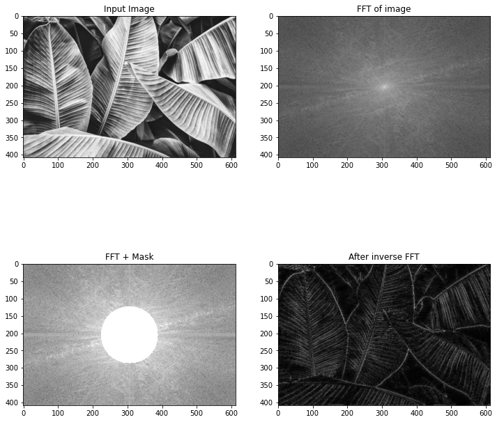
fshift = dft_shift * mask

Now we have an origin at the center of the image, so we need to move the origin back to the top left of the image. This is the undo process of dft_shift= np.fft.fftshift(dft)ft this shifting process already did.

f_ishift = np.fft.ifftshift(fshift)

Inverse DFT to convert back to the image domain from the frequency domain will be complex numbers

img_back = cv2.idft(f_ishift)

Magnitude spectrum of the image domain

img_back = cv2.magnitude(img_back[:, :, 0], img_back[:, :, 1])

Plotting the final results

fig = plt.figure(figsize=(12, 12))

ax1 = fig.add_subplot(2,2,1)
ax1.imshow(img, cmap='gray')
ax1.title.set_text('Input Image')
ax2 = fig.add_subplot(2,2,2)
ax2.imshow(magnitude_spectrum, cmap='gray')
ax2.title.set_text('FFT of image')
ax3 = fig.add_subplot(2,2,3)
ax3.imshow(fshift_mask_mag, cmap='gray')
ax3.title.set_text('FFT + Mask')
ax4 = fig.add_subplot(2,2,4)
ax4.imshow(img_back, cmap='gray')
ax4.title.set_text('After inverse FFT')

plt.show()

The final output program is present in the GitHub repository for reference.

Thank you for reading!

Reference :

Fourier transform