2D Multi-Person Pose Estimation using Part Affinity Fields in Computer Vision

Pose Estimation

Hello everyone, did you ever wonder while working out or playing sports if you’re doing it the right way? if this is how others do it?

Well, I have, and I kept thinking if I can use our dear friend AI to evaluate our performance.

The solution that I’ve arrived at is comparing the posture of two people to find out how it can be corrected.

This blog post is about my findings in the first step in solving this problem – POSE ESTIMATION.

In this post, we are going to discuss one of the most interesting problems in Computer Vision – Pose Estimation.

In particular, we’ll be looking at a brilliant paper “OpenPose: Realtime Multi-Person 2D Pose Estimation using Part Affinity Fields” [https://arxiv.org/abs/1812.08008]

Before we start, I would like to mention a few references that have helped me a lot in figuring out this intriguing problem, please have a look at them for better understanding. They are mentioned at the bottom of this blog in section 10.

Let’s dive in

1. What is it?

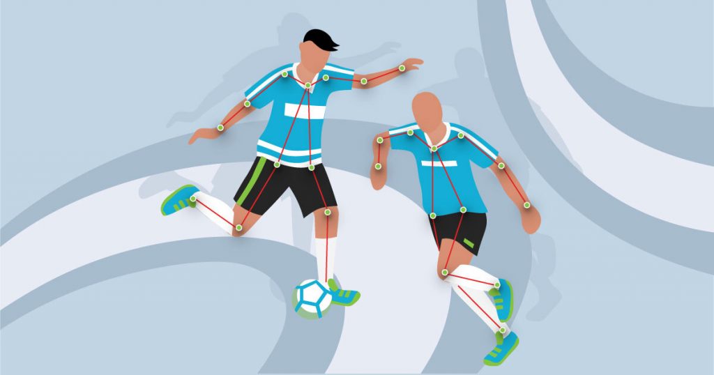
Pose Estimation is determining the pose of a person in an image. Which means we’ll be locating the joints and limbs in a person.

2D pose estimation is the determination of the pose of a person in a 2-Dimensional Space (X – Y coordinates).

2. Uses

Pose estimation can be used in many applications ranging from robotics and biomechanics (in order to correct the form and posture of a player) to predicting unusual activity in a live video stream

It can be used in animations even, to make the animation of human-like motion faster and simpler.

3. The Problem

Let’s look at this problem objectively, part by part. First, let’s define our problem statement

So, we have a standard image in RGB or BGR format, and we have to find out the location of certain body parts (Nose, Neck, Hip, etc.) in the image.

4. The Solution

So, how would one go about building a solution to this unique challenge?

Pose estimation is a familiar problem in the computer vision domain and many algorithmic approaches exist that can be used to solve this peculiar problem

We come across two common approaches: 1. Top-Down Approach, 2. Bottom-Up Approach

4.1 Top-Down Approach

The top-down approach is intuitive and is seemingly simpler, however, it can be computationally expensive in certain scenarios.

Let’s discuss this approach a little more before we reach any conclusions

Steps in TD Approach:

1. Find the people in an image using a people detector.
2. For each person run a deep neural network to detect the limb positions.

It is an intuitive and simpler approach however there are some pitfalls which can occur

1. What if a person is not detected in an image?

This happens in many conditions, for example, when one person is standing behind another, and due to certain orientations, or due to the background

There is no recourse to recovery and an entire limb connection configuration might be lost.

2. What would happen if there are 10 people in a frame?

The neural network should be run 10 times which is computationally expensive.

Let’s look at the bottom-up approach now.

4.2 Bottom-Up Approach

An excellent solution to the problems faced in the TD approach was provided in the Paper “OpenPose: Realtime Multi-Person 2D Pose Estimation using Part Affinity Fields” [https://arxiv.org/abs/1812.08008]

In the bottom-up approach that was proposed in the mentioned paper, the limbs are directly detected and are then paired to form an optimal configuration.

4.2.1 The overall pipeline of the method:

4.2.2 The Architecture of the proposed multistage CNN

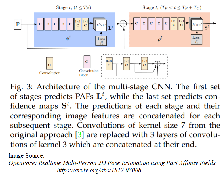
There are three important keywords in the pipeline and the architecture: Part Confidence maps, Part Affinity Fields and bipartite matching. We shall look at each of these in detail.

5. Part Confidence Maps

5.1 Part Confidence Maps

To show the working of the algorithm I’ll be using the open vino’s model based on OpenPose approach

The model documentation is available at https://docs.openvinotoolkit.org/latest/_models_intel_human_pose_estimation_0001_description_human_pose_estimation_0001.html

If we pass the input image through the OpenVINO neural network, it gives an output with two Matrices of shapes [1, 38, 32, 57] and [1, 19, 32, 57].

The first one is the key point pairwise relations AKA Part Affinity Fields and the second is the Part Confidence Maps.

What are Part Confidence Maps?

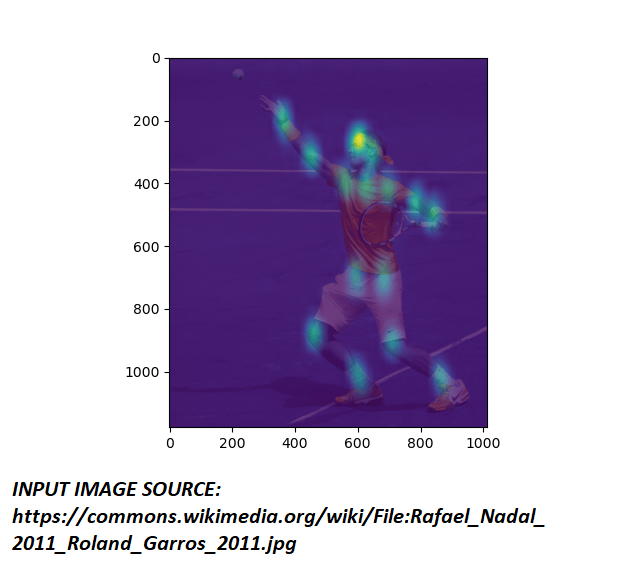
Part Confidence maps are heat maps that give the probability of a limb.

Combined Part Confidence Heat Map of figure 5.1 is shown in figure 5.2

Steps for Obtaining the key points from Part Confidences heat map

1. The output from the openvino net gives heatmaps of confidences in the shape [1,19,32,57].

Each of the 19 dimensions represents a single limb joint, the shape of the map is 32×57.

The 32×57 size map should be upscaled to the size of the frame to give more accurate results.

It can be done using simple cv2.resize, the interpolation technique INTER_CUBIC can be used for better accuracy however it is a complex process hence computationally expensive, it is a trade-off between time and accuracy.

2. Now we have a heatmap of size WxH W – width of the test image, H – Height of the test image.

We need to obtain the local maxima and apply a threshold to obtain the locations where a limb joint is present.

Note: Remember that this needs to be done 19 times for 19 limbs.

To achieve the task of finding local maxima I use a function peak_local_max from scikit image library

Example Code: loc_max = peak_local_max(heatMap, threshold_abs=conf_thresh)

3. Store this loc_max in a dictionary of parts {} where keys are the numerical index of the limb and values is a list of loc_max

Example:  if 0 represents Nose then dict_parts = {0: [(x1, y1), (x2, y2)]} if two noses are present

4. At the end of this step we have a dictionary with points of joints, let’s plot these on the image and see which one is which point

There are some errors in the output, we would want to remove these errors, let’s look at PAF now

6. Part Affinity Fields

Everything is well and good when we are working with images containing a single person, but what would be the output when we pass an input like figure 6.1?

The output would look like figure 6.2,

Now, how do we know which limbs belong to which person?

We cannot use distance measurement since that would give very inaccurate results when people are standing close to each other during social interactions.

This is where Part Affinity Fields come into play

6.1 Part Affinity Fields

Part Affinity Fields are nothing but direction Vectors of a limb, let’s visualize what these mean for better understanding

Did you notice how the number of dimensions of the PAF is twice that of Confidence Maps?

This is because for any 2D vector there are two components, one along X and one along Y

General representation goes with U and V, let’s see how to use these U and V vectors to visualize the direction of flow in a limb

Steps for visualizing PAF on an input image

1. For each limb connection, u and v are consecutive 32×57 maps
2. Upscale these maps to the dimension of the frame, like we did for confidence heat maps
3. Now we have u and v, let us draw these vectors using matplotlib quiver

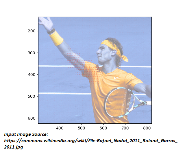
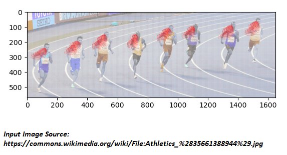
Notice how in Figure 6.3 the direction vectors U*-1 and V flow from elbow to shoulder.

7. Matching Algorithm

We have PAF and Peak values of joints. Let’s score each configuration.

The Open Pose paper suggests the use of a Greedy Algorithm approach to find out the best configuration

Steps in matching algorithm

1. Let’s start scoring each connection
2. Now, we pick all the elbows and all the shoulder points
3. We’ll be obtaining a matrix of dimension n_shoulder X n_elbow
4. FOR EACH CONFIGURATION CONTAINING ONE ELBOW AND ONE SHOULDER JOINT
   1. We construct a unit vector between the two points
   2. Consider n equidistant point between source and target peaks
   3. At least for 0.8*n points, the value of u and v should be > 0.01, else it doesn’t lie on a limb so return a negative value
   4. We’ll see how much is the difference in angle between the orientations of these two vectors ((ui + vj) and peak points vector).
   5. If these two are the same the output would be zero, however, we want it to be maximum for matching so subtract this value from 180. [180 – angle b/w two vectors].
   6. We do this because in the matching algorithm we select the maximum weight to the most feasible one
   7. To this add a distance score according to

norm = math.sqrt((src[0] - tar[0]) ** 2 + (src[1] - tar[1]) ** 2))
dist_score = min(0.5 * W / norm - 1, 0)
# where Src - shoulder, tar - elbow, w - width of the frame

5. To do the matching, I used a method max_weight_matching from the module Networkx which is a very useful module for graph-based algorithms.

Example Code: 

G = nx.Graph()
edges_list = []
for i, a in enumerate(source_limbs_peaks):
    for j, b in enumerate(target_limbs_peaks):
        edges_list.append((tuple(a), tuple(b), {"weight": score_matrix[i][j]}))
G.add_edges_from(edges_list)
matched = nx.algorithms.matching.max_weight_matching(G)
G.clear()

7. These are the matchings, store these connection links

8. Pairing the connections together

Let’s have a recap of what we calculated till now

We have all the peak locations – limb joint locations, we know which two joints are connected.

We now need to join these to form a complete set of human configuration

But how do we do that when we don’t know the number of people present?

Steps to assign each connection to a person

1. Let’s create a dictionary where keys = limbs & values = person_id
2. Initially all person_id = None
3. Let’s start with Neck or Nose, we know each person has only one. Whenever we encounter a None for person_id assign it the value of the number of persons and increase the number of people by one.
4. Now when we come to the connections between Neck and shoulder, for example, all necks will have a person_id assigned,  we’ll pass this id to shoulders i.e if neck-1 and shoulder-2 is a connection then neck-1 and shoulder-2 will have the same person_id.

5. For shoulder-elbow connections, if for any shoulder the person_id == None, we’ll assign it as a new person. This way, even if a neck is not detected, the rest of the configuration is saved
6. Now, delete the person lists with the number of joint elements less than 3

Now let’s display the results

9. Conclusion

Now that poses can be extracted, we can use this to correct the stance and form of an athlete or use it to predict unusual activities from a live stream.

It can be used for creating animated videos in software like Blender, and make the process of animating human-like motions simpler.

10. References

1. https://arxiv.org/abs/1812.08008
2. https://towardsdatascience.com/cvpr-2017-openpose-realtime-multi-person-2d-pose-estimation-using-part-affinity-fields-f2ce18d720e8
3. https://github.com/ZheC/Realtime_Multi-Person_Pose_Estimation/
4. https://github.com/CMU-Perceptual-Computing-Lab/openpose
5. https://docs.openvinotoolkit.org/latest/_models_intel_human_pose_estimation_0001_description_human_pose_estimation_0001.html

Please feel free to share your thoughts or any doubts in the comments section below 🙂